
Entity-Attribute-Value (EAV) Model: Examples and Tradeoffs
Learn how the entity-attribute-value (EAV) model stores flexible fields, where analytics counts go wrong, and how to prepare a reliable semantic model.
TL;DR
- Entity-attribute-value (EAV) stores changing properties as rows instead of adding a column for every possible property.
- That flexibility helps capture sparse data, but an attribute row is not an entity. Counting the wrong grain can inflate an analysis.
- Keep the flexible source when it serves the application; give recurring analysis a typed, tested, one-row-per-entity view and a reviewed semantic definition.
An entity-attribute-value model is a database pattern that represents each property as an entity ID, an attribute name, and a value. A customer can have a plan row and a region row rather than fixed plan and region columns. It accommodates properties that vary across customers. For analytics, the critical step is to turn those rows back into a clearly defined entity before counting or joining. See the short EAV glossary entry for the term at a glance.
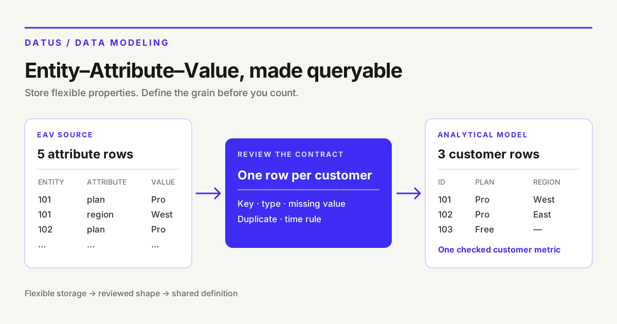
EAV is a storage choice. Analytical grain and metric meaning still need an explicit contract.
How the EAV pattern works
An EAV table typically has three logical fields: entity, attribute, and value. A separate entity table may hold stable fields such as customer_id and created_at. The attribute table carries properties that can differ by entity or change as a product adds custom fields. This is often called a vertical representation: properties that would be columns in a conventional table appear as multiple rows instead. The MariaDB EAV implementation guide describes the original motivation as an open-ended attribute set with mixed value types and ad hoc queries.
Suppose a customer application permits optional plan and region fields. This illustrative, hand-sized dataset shows the physical rows; it is not a product benchmark or a customer example.
customer_id |
attribute_name |
value_text |
|---|---|---|
| 101 | plan | Pro |
| 101 | region | West |
| 102 | plan | Pro |
| 102 | region | East |
| 103 | plan | Free |
The table has five attribute rows for three customers. Customer 103 has no region row; absence needs an agreed interpretation. If the attribute is optional, absence may simply mean unknown. It should not silently become “East,” “West,” or “not applicable.” The application can add a new property without adding a new physical column, but each analytical question must still decide which properties matter and how missing values behave.
A useful distinction is between an entity and a fact about an entity. customer_id = 101 identifies the customer. Its plan = Pro and region = West rows are two facts. They cannot both become two customers merely because a query joined them. This distinction is easy to preserve in application code that fetches one customer at a time. It is easier to lose when a reporting query starts from the attribute table.
Where EAV helps—and what it asks you to manage
EAV fits a genuinely open set of sparse, optional properties: custom form fields, heterogeneous catalog items, or research observations with different measurements. If only a small subset of all possible fields applies to each record, a fixed table can be awkward to evolve. The pattern makes adding a new kind of attribute largely a data operation. It can also preserve attributes whose business importance has not yet been decided.
The flexibility moves work elsewhere. The database does not automatically know that plan is a string with allowed values, trial_start is a date, and employee_count is numeric when all three sit in value_text. Text comparison can make a numeric range wrong: '100' and '20' sort differently as strings than 100 and 20 do as numbers. MariaDB’s guide flags both type handling and repeated self-joins as practical costs of a naive three-column implementation. Typed value columns, an attribute registry, or application validation can address some of these issues, but those rules must be maintained.
The table also needs a cardinality rule. Is one region allowed per customer, or can a customer have several? If the former, enforce uniqueness on (customer_id, attribute_name) for the applicable rows. If the latter, a pivot that selects one value is a business decision, not a harmless formatting change. Historical changes need an effective-time rule as well: “current region” and “region when the order happened” are different questions. Neither an EAV table nor a semantic layer can invent that rule after the fact.
| Design question | EAV source can store | Analysis must decide |
|---|---|---|
| Optional fields | No row for a missing attribute | Unknown, inapplicable, or a documented default? |
| Multiple values | Several rows for one attribute | Multi-valued field or data-quality error? |
| Types | Text, typed value columns, or referenced values | Which values are numeric, dates, or categories? |
| History | Repeated rows with timestamps | Current value or value at event time? |
| Identity | Attributes keyed to an entity ID | Which key and grain define a count? |
These are not arguments against the pattern in every case. They are the contract you need if other teams will query the data. A useful test is whether the attribute set is truly open or merely a small group of stable, frequently filtered fields. For the latter, ordinary typed columns may be simpler. MariaDB’s guide suggests keeping frequently searched properties as typed, indexed columns and storing less-used extras separately. That is one design option, not a universal migration recipe.
The counting error: five rows, three customers
The easiest EAV error to demonstrate is a count at the wrong grain. Suppose customers contains IDs 101, 102, and 103, and customer_attributes contains the five rows above. A left join followed by COUNT(*) answers “How many joined rows are there?” For this fixture the answer is five, even though there are three customers. More attributes per customer make the gap larger.
SELECT COUNT(*) AS joined_rows
FROM customers AS c
LEFT JOIN customer_attributes AS a
  ON a.customer_id = c.customer_id;
-- illustrative result: 5, not 3 customers
COUNT(DISTINCT c.customer_id) returns three here, but it is not a complete modeling strategy. A distinct count does not tell you which region to use if there are two rows for that attribute, whether a missing plan should count as Free, or which version of a value was in force on a past date. It can also conceal a broken join that affects sums and averages differently. Start by declaring the desired grain—one row per customer, one row per order, or one row per observation—then check every join against it.
For a recurring customer report, a curated one-row-per-customer dataset makes the grain visible. The following SQL is a small illustrative transformation over the fixture above. It assumes plan and region are each single-valued for a customer and that the source enforces that rule. It is not SQL emitted by Datus or Dosi.
WITH attributes_by_customer AS (
  SELECT
    customer_id,
    MAX(CASE WHEN attribute_name = 'plan' THEN value_text END) AS plan,
    MAX(CASE WHEN attribute_name = 'region' THEN value_text END) AS region
  FROM customer_attributes
  WHERE attribute_name IN ('plan', 'region')
  GROUP BY customer_id
)
SELECT c.customer_id, a.plan, a.region
FROM customers AS c
LEFT JOIN attributes_by_customer AS a
  ON a.customer_id = c.customer_id;
The result has three customer rows: (101, Pro, West), (102, Pro, East), and (103, Free, NULL). A query for Pro customers in the West now has an auditable answer: one. MAX is safe here only because each selected attribute has at most one value per customer. If that uniqueness check fails, the query silently chooses a value; fix the source contract or specify a deterministic rule before publishing the dataset. The Google Developer forum’s EAV analysis walkthrough also shows why flattening can help analytical queries, while noting that persistence and refresh choices depend on the workload.
This example is deliberately small, but the failure is not about table size. It is about meaning. An analyst who sees five rows and calls the result “customers” has changed the unit of analysis. The same issue arises when a dashboard or AI agent discovers the attribute table without a description of its grain. A semantic model can name the curated customer dataset and its key; it cannot rescue a source that has not resolved conflicting attribute values.
Before calling the reshaped dataset production-ready, make the assumption testable. The expected attribute keys in this fixture are plan and region; a new spelling such as customer_region should not quietly create another dimension. Check for duplicate (customer_id, attribute_name) pairs and for values outside the approved plan vocabulary. Confirm that every customer in the entity table appears in the view, even when no optional attributes exist. For a daily refresh, compare the number of distinct source customers with the number of published customer rows. A mismatch should block or flag the refresh until someone explains it. These checks turn the SQL’s implicit assumptions into an explicit data contract.
EAV, JSON, and typed columns answer different needs
The choice is not “flexible EAV or no flexibility.” A conventional entity table can keep stable fields as typed columns and reserve a JSON field for less predictable extras. PostgreSQL’s JSON type documentation explains that jsonb supports indexing, with different storage and write tradeoffs from json. The relevant database and query workload determine whether that is simpler than EAV. Neither format automatically tells a BI tool what a custom key means to the business.
| Shape | Often useful when | Analytical work still needed |
|---|---|---|
| Typed columns | The important fields and types are stable | Agree on business definitions and joins |
| EAV rows | Attributes are numerous, sparse, and change often | Enforce keys and types; select and reshape queryable fields |
| Entity row plus JSON extras | A stable core coexists with occasional custom fields | Decide which JSON keys become governed dimensions |
| Curated analytical view | A repeated report needs a stable grain | Test refresh, missing values, and metric rules |
A team may use more than one shape. The operational application can retain EAV for customization while a warehouse publishes a curated view for reporting. The view can include only approved fields, with explicit null handling and a documented refresh policy. That keeps storage flexibility from leaking into every downstream query. It also gives a clear place to validate the one-row-per-entity invariant before an agent or dashboard uses it.
The decision changes with use. If only one application reads a record by ID and displays its custom fields, EAV may serve that workflow well; building a second analytical model for a report no one needs adds maintenance. If many consumers repeatedly ask for “Pro customers by region,” the stable view earns its upkeep. If the attributes themselves are events or observations, a one-row-per-customer pivot may erase important detail; model the observation grain instead. The goal is to publish the shape appropriate to the question, not to flatten every EAV table by default.
Make the analytical contract available to agents
An AI agent looking at customer_attributes might see customer_id, attribute_name, and value_text, but not the single-valued rule, the approved plan vocabulary, or the report’s grain. Those facts belong in reviewed context, alongside the queryable dataset. Schema linking helps identify relevant tables and columns; it does not by itself determine whether an attribute row represents a customer. For an agent answering “How many Pro customers are in the West?”, the safe path is to use the curated customer dataset or an approved metric, then check the result against the fixture above.
As of October 2026, Datus’s semantic-model documentation describes datasets backed by a physical table or a reusable SQL query, with fields, relationships, verified keys, and metrics in the model. That supports modeling a stable customer view or query result after the EAV-specific transformation has been defined and reviewed. It does not mean Datus automatically decides how to pivot arbitrary custom attributes or which conflicting value wins. A model author still has to establish those rules and validate representative queries.
The wider semantic layer supplies a shared place for those definitions across tools. In an EAV setting, this is especially useful because physical names alone carry so little business meaning. A dataset named customer_profile with a verified customer_id key, a defined plan dimension, and a reviewed customer_count metric offers an agent a clearer choice than a free-form instruction to join any row whose attribute_name seems relevant. The source can stay flexible; the answer needs a stable meaning.
Before exposing an EAV-backed metric, review a compact fixture: a customer with two attributes, one missing an attribute, one with a second value for a supposedly single-valued field, and one whose value changes over time. Assert the expected count and breakdown for each case. The semantic model examples post shows how to check a model against expected answers; this EAV case adds the source-shaping and cardinality checks that must happen first.
A practical decision checklist
If you are designing a new source, first ask whether the attributes are genuinely unpredictable or whether a handful of typed columns covers the reporting needs. For an existing EAV source, document the entity key, allowable attributes, value types, missing-value meaning, duplicate policy, and history rule. These decisions make the table queryable without pretending it is a conventional entity table.
Next, choose the analytical grain for each use case. Build a view or transformation only for the attributes you need to publish, and test that it produces one row per intended entity—or intentionally retains one row per observation. Validate counts before and after joins. Then place approved names, dimensions, keys, and metric rules in the semantic model. When an attribute is added or its meaning changes, update the transformation and its result-level tests together.
This sequence protects both flexibility and accuracy. The application can keep adding custom fields; analysts are not forced to rediscover the same pivot, type conversion, and duplicate rule on every query. More importantly, the model can say which questions the curated dataset actually answers and which ones still need the raw attribute history.
Conclusion
EAV is useful when entities carry varied, sparse properties. Its central analytics risk is a grain mismatch: rows about customers are mistaken for customer rows. Preserve the flexible source where it helps, but publish a tested analytical shape with typed fields, clear cardinality, and reviewed metric definitions for questions that recur. That is what lets people and agents count the same thing.
Frequently asked questions
What is an EAV model in a database?
An EAV model stores properties as rows with an entity identifier, an attribute name, and a value. It is useful when the set of possible properties changes or only a few properties apply to each entity. A separate table often stores stable entity fields. The pattern describes physical storage; it does not define the grain or business rules for an analytical metric.
When should I use EAV instead of regular columns?
Use it when attributes are genuinely open-ended and sparse enough that maintaining a fixed column for every possible property is awkward. If the important fields are stable and routinely filtered, typed columns are often easier to validate and query. Consider who reads the data: a custom-field application and a recurring customer report have different needs. A curated analytical view can serve the report while the application retains EAV.
Why can EAV produce the wrong count in a dashboard?
One entity can have many attribute rows. Joining an entity table to its attributes multiplies rows; COUNT(*) then counts joined rows rather than entities. In the example above, five attribute rows describe three customers. Declare the desired grain first, check join cardinality, and use a one-row-per-entity dataset or an explicitly defined distinct-entity metric. Resolve duplicates and time rules separately.
Is JSON better than an EAV table?
Neither is universally better. JSON can keep occasional custom properties beside stable entity columns, and some databases support indexing into it. EAV can make individual attributes explicit rows, which may suit a different write or query pattern. Compare your database’s type support, indexes, update behavior, and queries. Either way, promote recurring analytical fields into a governed, typed contract rather than asking every consumer to interpret raw keys.
Can a semantic layer query EAV data directly?
It can use a table or a reusable query if the model and engine support that source, but a semantic layer still needs the intended grain, key, field types, and business rules. For recurring entity metrics, a curated view or stable query result is usually easier to review than raw attribute rows. In Datus, the documented semantic model can map such a dataset; the EAV reshaping and validation remain explicit work for the team.
Related articles
- What is a semantic model? — define the dataset, keys, dimensions, and metrics that consumers share.
- Semantic model examples — inspect a tested model and its expected answers.
- What is schema linking? — see how agents identify relevant physical sources.